Demographic survey analysis software for Indian data
Three years ago, I sat with a district health officer outside Nashik, working through why two neighbouring blocks reported strikingly different institutional delivery rates despite near-identical infrastructure.
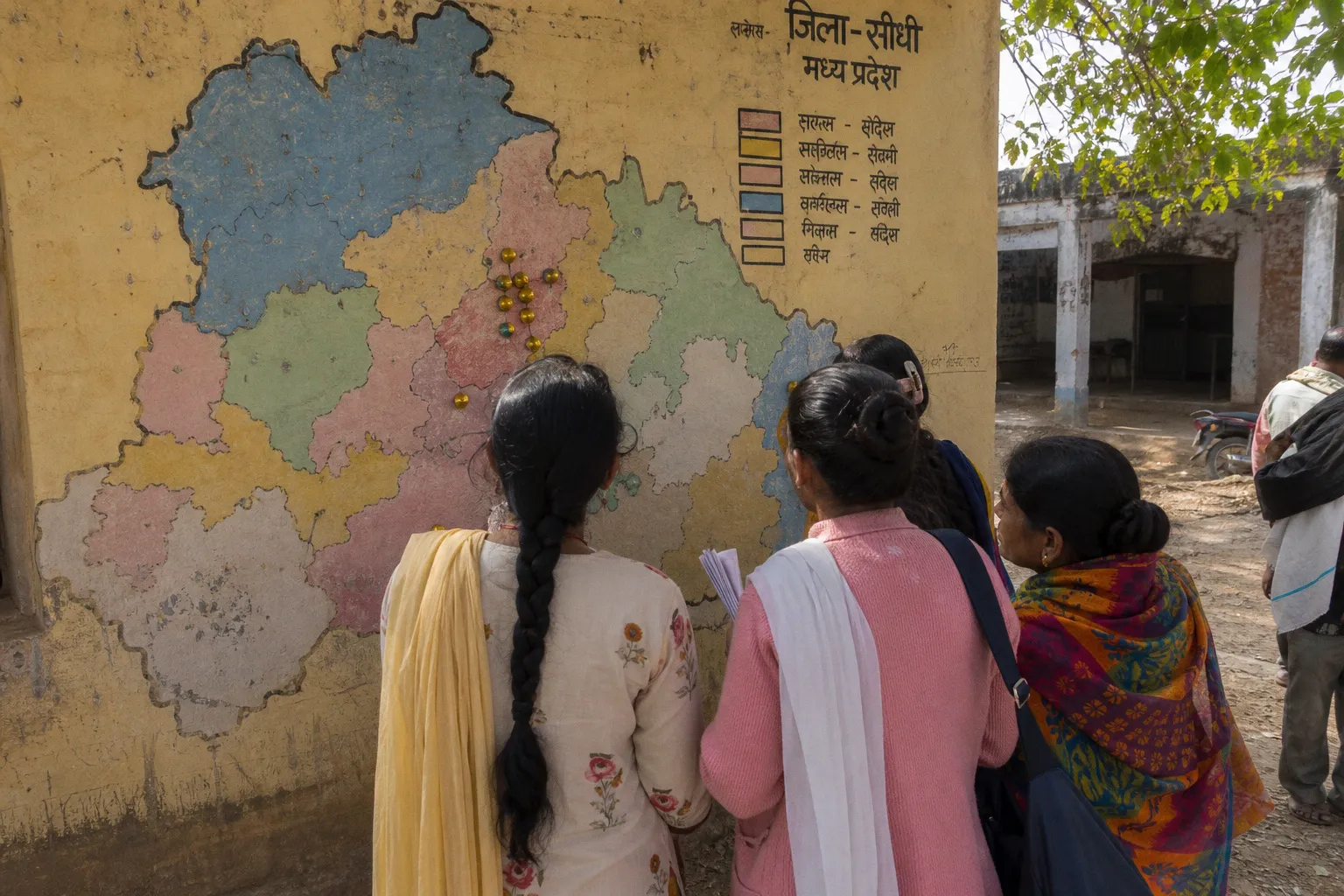
The NFHS-5 figures told one story, the clinic registers told another, and the gap between them sat squarely inside the survey analysis software chain — from CSPro cleaning routines through to the Stata regression syntax that produced the published estimates. That experience reframed how I read Indian demographic data: every number is the output of a tool stack, and the tools deserve to be understood on their own terms. What follows is a practitioner's map of that stack, written for clinicians, programme officers, and curious students who need the indicators to mean something at the bedside, not just in a journal.
Compare car rental deals in United Kingdom
See available offersPartner link — DiscoverCars comparisonData Entry and Cleaning: The Role of CSPro in Indian Surveys
CSPro — the Census and Survey Processing System — sits at the very front of the demographic survey pipeline, and in India it has been the workhorse for major household surveys for years. When the International Institute for Population Sciences (IIPS) in Mumbai, established in 1956 and declared a deemed university in 1985, plans a round of the National Family Health Survey (NFHS) or the District Level Household Survey (DLHS), CSPro is the system that handles data entry, primary editing, and secondary editing across hundreds of thousands of household interviews. It is also the system that produces the hierarchical files that eventually get converted into the flat Stata, SPSS, or SAS datasets that most downstream analysts actually open.
To put the scale in perspective, DLHS-3, with fieldwork in 2007–08, covered 601 districts and sampled 7,20,320 households. NFHS-5, conducted between 2019 and 2021, drew a comparable volume of responses from eligible women aged 15–49 and, in earlier rounds, eligible men aged 15–54. CSPro is what makes that scale manageable — it provides batch editing, range checks, consistency checks, and skip-pattern logic that mirror the questionnaire's structure. The microdata that eventually lands in your.dta or.sav file has usually been through at least two rounds of CSPro cleaning before you ever see it, and the documentation in NFHS final reports describes those checks in unusual detail.
For practitioners who rarely touch the raw entry layer, this still matters. The quality of any downstream analysis — whether you are modelling fertility decline, antenatal care coverage, child immunisation gaps, or adolescent reproductive health behaviour — is bounded by how well the upstream cleaning was done. When you see a suspiciously tidy variable, an oddly truncated age distribution, or a missing category that "just happens" to align with a skip rule in the questionnaire, CSPro's secondary editing routines are often the reason.
CSPro is not where statistical insight happens, but it is where honest statistical insight becomes possible.
Statistical Powerhouses: Comparing Stata, SPSS, and R for NFHS Microdata
Once the data is clean, the analytical conversation begins. For researchers, students, and analysts working with Indian demographic and health survey microdata, three names come up again and again: Stata, SPSS, and R. None of them has displaced the others; all three are actively taught and used at institutions like IIPS Mumbai and across public health training programmes in India. The choice between them usually reflects your training, your institution's licence agreements, and the kind of question you are asking.
What I have observed on the ground is that Stata remains a default in many Indian demographic research settings, partly because its 'svy' command prefix was designed specifically for complex survey data and partly because the syntax is forgiving for analysts coming from clinical backgrounds. SPSS holds strong in state health departments and surveillance units, where the graphical interface is more approachable for clinicians moving into data work and where complex samples modules are already licensed. R has grown rapidly in academic settings, especially where reproducibility, custom graphics, and the broader ecosystem of packages matter — and where the budget simply does not stretch to commercial licences.
NFHS microdata is distributed in multiple formats to accommodate exactly this split: Stata (.dta), SPSS (.sav), SAS transport files, and hierarchical CSPro files. The table below sketches the trade-offs I have watched researchers negotiate.
| Practical dimension | Stata | SPSS | R |
|---|---|---|---|
| Native handling of complex survey designs | Strong via the 'svy' command prefix | Strong via the Complex Samples module | Strong via the 'survey' package; most flexible for non-standard designs |
| Learning curve for clinicians entering data work | Moderate | Gentle at first, steeper for advanced scripting | Steepest, but pays off in reproducibility |
| Graphics and publication-ready output | Good via 'estout', 'coefplot', and successors | Functional, less customisable | Excellent via 'ggplot2', 'sf', 'tmap' |
| Cost and licensing | Paid licence, often institutional | Paid licence | Free, open source |
| Best fit for | Standard NFHS/DLHS regression tables and IIPS-style theses | State programme dashboards and clinician-led analyses | Custom modelling, geospatial joins, open-science workflows |
A common misstep I have seen junior analysts make is treating these three as interchangeable. They are not. Stata and R can both handle a complex survey design correctly, but the way you specify PSU nesting, the stratum variable, the finite population correction, and the weight variable differs in ways that matter when you publish or compare results across studies.
Accounting for Complex Survey Designs: Weights, Strata, and PSUs
This is the part of any NFHS or DLHS analysis where most clinical readers' eyes glaze over — and yet it is exactly where the numbers either deserve our trust or quietly mislead us. The District Level Household Survey, like NFHS, is not a simple random sample. It uses a stratified, multi-stage cluster design, with districts often serving as explicit strata, villages or urban blocks as primary sampling units (PSUs), and households selected within PSUs. Every household and every individual in the public-use file comes with a sampling weight that reflects how likely they were to be selected at each stage and how the design adjusted for non-response.
If you ignore those weights, you will produce estimates that look precise and are quietly wrong. A district-level anaemia prevalence calculated without the survey weight will treat every respondent as equally important, even though some represent 80 households and others represent 200. A regression of antenatal care visits on maternal education run without the 'svy' or 'survey' prefix will produce standard errors that are typically too small — the design effect is real, and in clustered health data it can easily push your confidence intervals into misleading territory.
In R, this is handled through the 'survey' package by Thomas Lumley, where you declare the PSU variable, the strata, and the weights explicitly before any model is fit. In Stata, the 'svyset' command followed by the 'svy:' prefix does the equivalent job at the top of your do-file. SPSS uses the Complex Samples analysis pathway through its menus and syntax. The specific syntax varies, but the underlying principle is identical: the software needs to know the sampling structure before it can give you estimates that reflect what was actually done in the field.
What this means for a clinician sitting in a district programme review meeting is straightforward. If you are quoting a district-level figure from a published analysis, ask whether the authors accounted for the complex survey design. If they ran an ordinary logistic regression on weighted data without setting the survey design, the confidence intervals are not what you think they are. This is not an academic quibble — it changes which districts you prioritise for outreach, which ASHA worker density estimates you trust, and which maternal mortality comparisons you take to the state office.
The right tool is the one that respects what the data can actually answer, and the question you are actually asking.
Specialised Demographic Modelling: MORTPAK and Spectrum Applications
Beyond the general-purpose statistical packages, the Indian demographic community relies on two more specialised tools that deserve a place in any honest toolkit. The first is MORTPAK, a software package developed by the United Nations that demographers use specifically for mortality measurement and the construction of abridged life tables. When DLHS or NFHS data is used to estimate infant mortality, under-five mortality, or adult mortality at the district level, MORTPAK is often the engine behind the scenes. It handles the smoothing of death rates, the construction of life tables from incomplete vital registration, and the indirect estimation techniques that are necessary when civil registration systems in a district are weak or partial.
The second is Spectrum, a policy modelling suite used to project population dynamics and explore demographic windows of opportunity. For India, this is not an abstract exercise: projections built using Spectrum have estimated India's demographic window of opportunity to span roughly 2011 to 2041 — the period during which the working-age share of the population is largest relative to dependents. Underlying those projections is a long-horizon demographic model with a base period around 2001 and forward projections that extend to 2061 and beyond. Understanding that window, and how it varies by state, depends on software that can model fertility decline, mortality change, and migration simultaneously.
For a clinical reader, the practical relevance is twofold. First, when state-level maternal mortality ratio estimates or neonatal mortality projections appear in policy documents and state action plans, they almost certainly came through MORTPAK, Spectrum, or both. Knowing this lets you read the numbers with appropriate humility and with awareness of the modelling assumptions behind them. Second, if you are involved in district-level planning, these tools are often accessible through IIPS Mumbai training programmes and through UNFPA-supported workshops — they are not proprietary secrets locked away from frontline practitioners.
Visualising District-Level Trends: GIS Integration and Spatial Analysis
The final layer of the toolkit, and the one that has changed most visibly in the past decade, is geospatial analysis. India has more than 600 districts, and a maternal health indicator that looks moderate at the national level can mask enormous intra-state and intra-district variation. The shift from coarse state-level dashboards to granular district-level mapping has been driven by software tools like ArcGIS, QGIS, and GeoDa, alongside R's 'sf' and 'tmap' packages and Python's geospatial stack.
ArcGIS remains the commercial standard in many government and planning settings, but QGIS — open source and increasingly capable — has become a realistic option for academic and NGO analysts working with limited budgets. GeoDa is particularly useful for exploratory spatial analysis: it makes it easy to spot clusters of high or low coverage, to compute local indicators of spatial association, and to test whether the patterns you see are likely to be chance. R's 'sf' package, paired with district shapefiles from the Survey of India or the DataMeet community, allows analysts to keep the entire workflow — from import to modelling to map — inside a reproducible script.
The honest caveat is that geospatial analysis on survey data requires care. NFHS and DLHS cluster locations are typically displaced for confidentiality, often by several kilometres, and the district identifiers in the public-use files are what most analysts actually map. Joining those identifiers to district shapefiles and visualising antenatal care coverage, full immunisation coverage, or the proportion of births attended by a skilled provider is straightforward; claiming that the resulting map shows precise intra-district hotspots is, more often than not, a misreading of what the underlying cluster design can support.
Choosing Your Stack
If I am asked, as I often am by midwifery students and junior programme officers, what software to learn first, the answer I give is shaped by what they actually want to do. For a clinician whose primary aim is to read and lightly analyse published survey findings, SPSS is the most forgiving entry point, and the NFHS microdata ships in a format that opens directly. For a researcher intending to publish theses, working papers, or peer-reviewed articles, Stata is the path of least resistance in the Indian demographic ecosystem — its 'svy' commands map directly onto what NFHS and DLHS documentation expects, and most IIPS faculty and supervisors are fluent in it. For anyone interested in reproducible workflows, custom modelling, geospatial joins, or the open-science side of population analytics, R is worth the steeper climb and a long-term investment.
Three things I would urge anyone analysing Indian demographic survey data to keep in mind, regardless of which software they choose:
- Set the survey design before you run any model — declare the PSUs, strata, and weights, and treat this as a non-negotiable first step that conditions everything that follows.
- Match your tool to the question, not the other way round. A simple descriptive table is fine in any of the three; a hierarchical spatial model is not, and forcing it into the wrong software produces brittle results.
- Stay close to the original documentation. NFHS and DLHS final reports are unusually generous with their methodology appendices, and reading them carefully will save you from the most common analytic errors.
The Indian demographic survey ecosystem is unusual in how openly it publishes both its data and its methodology, with recruitment and preparation for NFHS-6 already underway. The tools described here — CSPro for entry and editing, Stata, SPSS, and R for analysis, MORTPAK and Spectrum for demographic modelling, and the GIS layer for spatial interpretation — are the same ones used by the people who design the surveys. Learning to work with them is, in a real sense, learning to read the evidence base of maternal and child health in India on its own terms.