DLHS and NFHS data anomalies: how to avoid analysis traps
DLHS-3 was completed across 601 districts. NFHS-5 reports results for 707 districts. Treating those two counts as a continuous district series produces a false panel before a single indicator has been calculated.
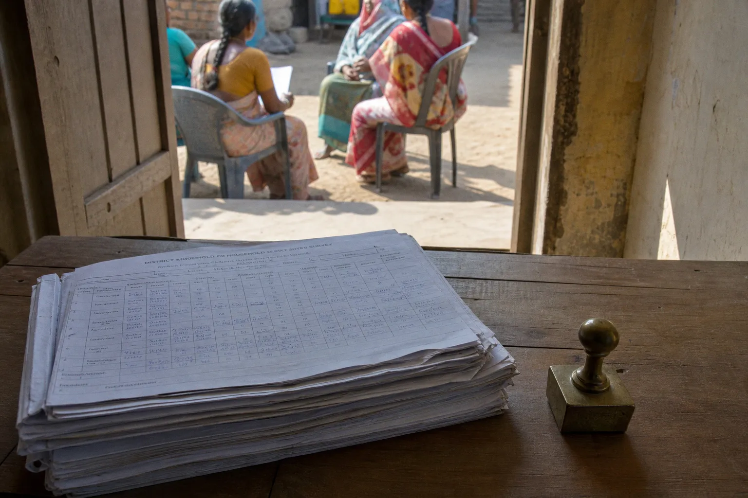
This is the central problem in DLHS and NFHS indicator discrepancies. Most visible divergences are not evidence of deteriorating services, improved outcomes, respondent error, or institutional manipulation. They are often the expected output of different sampling frames, eligibility rules, district boundaries, questionnaire modules, and weighting systems. A percentage is not self-explanatory. Its denominator, geography, reference period, and design determine what it measures.
The District Level Household Survey series remains indispensable for reconstructing India’s reproductive and child health landscape from the late 1990s through 2012–13. NFHS provides the more integrated contemporary architecture. Neither series is defective because it does not reproduce the other. The analytical failure begins when an investigator assumes that identical labels imply identical estimates.
The methodological divide: similar indicators, different survey objects
DLHS rounds were designed around district-level monitoring of reproductive and child health services. NFHS is a broader demographic and health survey system, built to estimate population, fertility, morbidity, nutrition, and service-use indicators across national, state, and district levels. The overlap is substantial. The equivalence is not.
The historical sequence matters:
| Survey round | Field period | District architecture relevant to analysis | Core implication |
|---|---|---|---|
| DLHS-1 | 1998–99 | Early district-level RCH monitoring | Baseline geography predates later district proliferation |
| DLHS-2 | 2002–04 | District estimates continued | Not automatically comparable with later district boundaries |
| DLHS-3 | 2007–08 | 612 districts sampled; data completed in 601 districts | Uses the 2001 Census sampling frame |
| DLHS-4 | 2012–13 | Final DLHS round | Transitional point before integrated NFHS approach |
| NFHS-4 | 2015–16 | 640 districts, aligned to the 2011 Census-era structure | Different district vintage from both DLHS-3 and NFHS-5 |
| NFHS-5 | 2019–21 | 707 districts, defined as of March 31, 2017 | Fieldwork spans pre-COVID and COVID-period observations |
DLHS-3 itself used distinct designs in rural and urban settings. Rural areas followed a two-stage stratified random design. Urban areas used a three-stage stratified design. Primary sampling units were drawn from the 2001 Census frame. The design is not a technical footnote. It determines clustering, stratification, variance, and the population to which an estimate can be generalized.
NFHS-5 employed a uniform design intended to yield estimates for India, states and union territories, and districts. It reached 636,699 households, 724,115 women aged 15–49, and 101,839 men aged 15–54. The achieved scale is large. It does not erase the need for design-aware inference at the district level.
A direct comparison is defensible only after the analyst specifies the actual comparison object. “Institutional delivery in District X” is not yet an object. It becomes one only after defining:
- the eligible women;
- the birth reference period;
- the exact questionnaire item and tabulation rule;
- the district boundary vintage;
- the survey round and fieldwork period;
- the applicable survey weight and design specification.
Without these conditions, an apparent trend is merely a subtraction.
A difference between two published percentages is not a trend until the two percentages describe the same population under comparable measurement rules.
Denominator dynamics: the most common source of false change
The most consequential DLHS–NFHS mismatch is often hidden in the denominator.
DLHS-3 interviewed ever-married women aged 15–49 and never-married women aged 15–24. NFHS-5 interviewed all women aged 15–49. This difference is sufficient to alter estimates for indicators related to knowledge, service use, fertility preferences, marriage, contraception, and exposure to reproductive-health questions. An analyst who extracts an NFHS-5 estimate from the complete women’s file and sets it beside a DLHS-3 estimate may be comparing overlapping but non-identical universes.
The error is easy to make because indicator labels are short. “Current use of contraception,” “unmet need,” or “awareness of HIV/AIDS” can appear stable in a spreadsheet while their eligibility logic has shifted. Published fact sheets may also apply tabulation restrictions that are not visible in a variable name.
The denominator should be reconstructed before the numerator is interpreted. In practice, this means reading the survey documentation and identifying whether the indicator applies to:
1. all women aged 15–49;
2. ever-married women aged 15–49;
3. currently married women;
4. women with a live birth in a defined recall period;
5. mothers of children in a particular age range;
6. households, children, men, or another eligible cohort.
This is especially material for RCH data indicators longitudinal analysis. Service-use measures commonly depend on a recent birth cohort. Fertility measures may depend on all women, currently married women, or birth histories. Child health estimates depend on surviving children, age windows, and in some cases a subsample. A label does not preserve these distinctions.
The correct procedure is not to force both surveys into a nominally common denominator if the underlying questionnaire cannot support it. The correct procedure is to identify the narrowest valid common population. If that population cannot be constructed, the indicator should be reported as non-comparable rather than converted into a spurious time series.
Recall periods can create a second denominator
The calendar year of fieldwork is also not necessarily the year of the outcome. A maternal-care indicator may refer to births occurring several years before the interview. A morbidity measure may use a recent recall window. A nutrition indicator reflects measurement at interview. These are different temporal objects.
NFHS-5 fieldwork ran from June 17, 2019 to April 30, 2021, across two phases. Its district estimates therefore combine observations collected before and during the COVID-19 period. A result published under the label “2019–21” should not be treated as a measurement from a single epidemiological moment. This is particularly relevant for facility delivery, antenatal care contacts, immunisation, and reported morbidity indices, where service availability and household mobility were disrupted unevenly.
A comparison between DLHS-4 and NFHS-5 may thus include both a survey-system transition and a fieldwork-period disturbance. Neither should be collapsed into a simple narrative of progress or decline.
Geographic evolution: district names are not district units
District boundaries are administrative variables. They change. Names persist, split, merge, and migrate across state structures. Name matching is therefore an inadequate method for assembling longitudinal district data.
DLHS-3 was based on the 2001 Census sampling frame. NFHS-4 covered 640 districts corresponding to the district structure at the time of the 2011 Census. NFHS-5 covered 707 districts, with its universe defined as of March 31, 2017. These are three different geographic reference systems.
The practical implication is direct: a district-level estimate from DLHS-3 cannot be linked to NFHS-5 solely because both records contain the same district name. The population base may differ. The land area may differ. The urban-rural composition may differ. A newly created district can remove higher- or lower-risk blocks from the parent district, changing the estimate even if individual behavior has not changed.
A defensible geographic workflow has three stages:
1. Freeze the target geography. Select one administrative vintage as the reporting framework. For long-run analysis, this is usually the older geography or a higher administrative level such as the state.
2. Build a documented crosswalk. Map each historical district to the target unit using explicit split, merger, and boundary-change rules. Retain one-to-many and many-to-one mappings rather than concealing them.
3. Aggregate before comparison where necessary. If a DLHS district split into several NFHS-5 districts, aggregate the later estimates to the parent geography using appropriate population or survey-weighted methods. Do not average percentages across successor districts.
The last point is routinely mishandled. An unweighted mean of district percentages gives a small district the same influence as a large one. This does not recreate the parent district estimate. It creates a new statistic with no clear population interpretation.
For some analyses, the best decision is to abandon district-level comparison. State-level harmonisation may preserve validity better than a district panel assembled through speculative crosswalks. Geographic granularity is not an achievement if the unit is unstable.
District-level precision does not compensate for district-level non-equivalence.
Weighting and module constraints: published estimates cannot be reproduced by raw counts
NFHS-5 provides separate weights for different units of analysis. The household weight, commonly identified as hv005, is intended for household indicators. The women’s individual weight, v005, is used for women’s indicators. These weights operate at national, regional, state, and district levels according to the relevant analysis plan.
A raw microdata tabulation is therefore not a replication of a published NFHS fact-sheet estimate. It is an unweighted sample proportion.
The discrepancy can be substantial in districts with unequal selection probabilities, differential response, or a sample distribution that differs from the population distribution. Weighting corrects the estimator for the survey design. It does not merely make the result look official.
The minimum analytical specification for a district estimate should include:
- the correct unit-level analysis weight;
- strata and primary sampling units;
- the survey round’s clustering structure;
- the eligible population restriction;
- the indicator-specific numerator and denominator;
- a survey-design-based standard error or confidence interval.
The final item is frequently omitted. It should not be.
DLHS-3 district samples were deliberately unequal: 1,500 households in low-performing districts, 1,200 in medium-performing districts, and 1,000 in good-performing districts. The classification was based on DLHS-2 information. Nominal district sample size, therefore, was partly related to prior district performance. Precision is not uniform across districts.
A change of three percentage points can be analytically empty when confidence intervals overlap widely or when design effects inflate the standard error. Conversely, a smaller change can be statistically distinguishable if the estimate is precise. Ranking district movements without uncertainty intervals produces a league table, not a finding.
Not every NFHS-5 indicator is a district indicator
NFHS-5 also divides its women’s questionnaire across district and state modules. The district module covered the household questionnaire and women’s questionnaire through section 7. The state module covered the full women’s questionnaire through section 11.
This means that a variable may exist in the NFHS-5 women’s file without supporting a district-representative estimate. Presence in microdata is not evidence of district-level validity.
This is a recurrent failure in demographic health surveys India data cleaning. Analysts identify a variable, filter to a district, apply a weight, and assume the output is a district estimate. The calculation may be syntactically correct and statistically invalid. The relevant question is not whether a variable can be tabulated by district. It is whether the sample design supports district inference for that variable.
The same caution applies when comparing IIPS Mumbai reports across rounds. A state report, district fact sheet, national report, and microdata file may contain overlapping statistics but not necessarily identical estimation universes or tabulation procedures. The report title is not the methodological specification.
Beyond sampling: data quality affects denominators before analysis begins
Not all district level household survey data errors originate in the sampling design. Non-sampling error can alter eligibility, reporting, and derived variables.
Age reporting is a concrete example. A published assessment of DLHS-3 data quality examined age reporting because an incorrect age in the household questionnaire could exclude a woman from the individual interview eligibility range. If a woman aged 49 is recorded as 50, she may be omitted from the eligible population. If a younger respondent is misclassified around another threshold, subgroup distributions can shift.
This is not a minor data-cleaning issue. It affects the denominator before any reproductive-health indicator is calculated.
Other non-sampling risks include interviewer effects, response error, missingness, translation differences, changed question order, and household roster inaccuracies. These cannot be solved by weighting alone. Weighting addresses known design and response structures. It does not reconstruct answers that were never collected or make two differently worded questions identical.
The appropriate response is an audit trail rather than retrospective certainty. For each indicator, retain a compact metadata record:
| Metadata field | Why it matters |
|---|---|
| Survey round and fieldwork dates | Defines the observation period |
| Source file and variable names | Allows replication and review |
| Eligible population | Establishes the denominator |
| Numerator rule | Prevents label-based assumptions |
| Recall period | Locates the outcome in time |
| Geographic vintage | Prevents false district matching |
| Weight and design variables | Supports valid point estimates and uncertainty |
| Questionnaire module | Confirms the valid level of inference |
| Comparability status | Separates harmonised trends from descriptive parallels |
This record is not administrative overhead. It is the minimum evidence required to defend an estimate after a report is published.
A restrained protocol for longitudinal RCH analysis
A useful longitudinal file should contain fewer indicators than a maximal extraction. The objective is comparability, not volume.
Start with an indicator inventory. Classify each candidate measure as fully harmonised, partially harmonised, non-comparable, or unavailable at the desired geographic level. “Partially harmonised” should be used sparingly. It means the difference is explicit and analytically bounded, not merely inconvenient.
Next, calculate estimates independently within each survey round using that round’s documented design. Do not pool DLHS and NFHS microdata into a single file and apply one common weight. The surveys have different frames, stages, selection probabilities, and field procedures. Pooling may be possible for a narrowly defined model, but only with a survey-specific design specification and a clear inferential target.
Then present the results in layers:
- Comparable estimates can be shown as a trend, with confidence intervals.
- Related but non-identical estimates should be presented side by side, with the denominator difference stated in the table note.
- Invalid district comparisons should be suppressed or aggregated to a stable geography.
- Variables outside the NFHS district module should not be reported as district-representative.
This approach is less visually dramatic. It is methodologically usable.
The alternative is familiar: a chart showing a steep rise or fall, a district ranking, and a causal explanation appended after the fact. Such charts often reflect changes in the measurement system more clearly than changes in population health.
The correct conclusion is often narrower than the first result
DLHS and NFHS were not designed as interchangeable annual accounting systems. They are large, complex survey programmes operating across changing administrative maps and evolving health-information needs. Their differences carry information about the survey architecture. They do not automatically reveal an anomaly in the population.
For analysts working with fertility, maternal health, child health, or service coverage, the first output should not be a district trend line. It should be a comparability decision. Is the population the same? Is the geography the same? Is the question the same? Is the weight appropriate? Is the estimate district-representative? Is the apparent change larger than its uncertainty?
If the answer to any of these is no, the result should be narrowed, qualified, aggregated, or withheld.
India’s next generation of population analytics will depend less on extracting more percentages from household surveys than on preserving the conditions under which those percentages remain interpretable. The strongest finding is not the largest observed difference. It is the difference that survives denominator harmonisation, geographic reconciliation, survey-design estimation, and scrutiny of the underlying measurement process.