DLHS dataset merging: a step-by-step researcher roadmap
DLHS-3 contains records from 720,320 households and 643,944 ever-married women aged 15–49. Those figures alone rule out casual file handling.
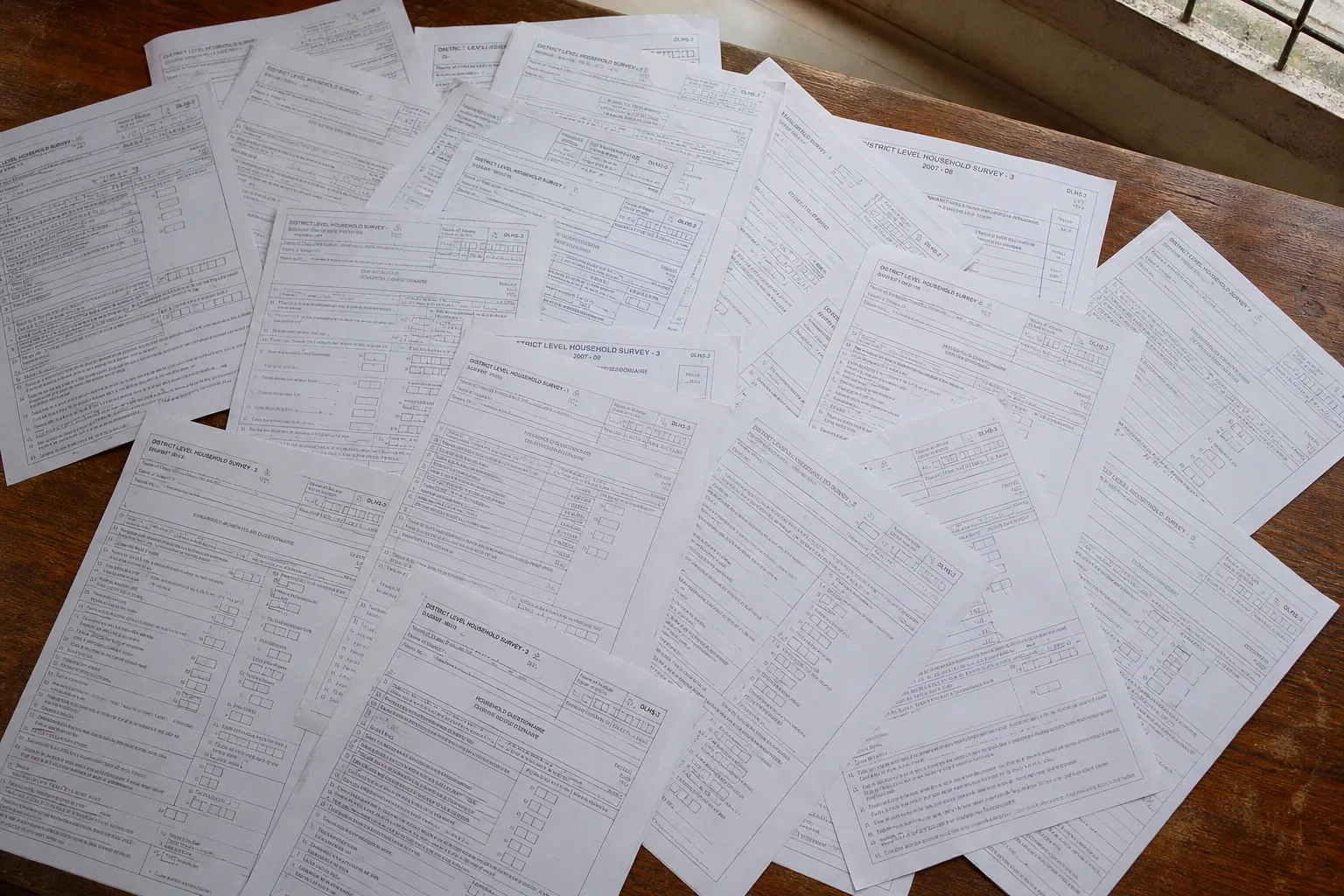
A merge that drops even a modest fraction of women, duplicates households, or applies the wrong weight can alter district estimates without producing an obvious software error.
The central fact is structural. DLHS household and individual data are nested. The household roster is collected first. Eligible women are then interviewed within the sampled household. Household characteristics therefore belong at one level; reproductive, maternal-care, child-care, and contraception outcomes belong at another. Treating these files as a one-to-one pair is not a technical shortcut. It is a unit-of-analysis error.
DLHS household and individual dataset merging should begin with a declared analytic population: households, ever-married women, unmarried women where applicable, births, children, facilities, or villages. The base file, identifiers, merge direction, and weights follow from that decision.
Understand the nested architecture before opening the merge dialog
DLHS rounds did not use an interchangeable file architecture.
DLHS-1 was conducted in 1998–99, DLHS-2 in 2002–04, DLHS-3 in 2007–08, and DLHS-4 in 2012–13. These are related survey programmes, not automatically harmonized longitudinal files. Each round must be inspected on its own documentation, questionnaire set, variable labels, field universe, geography, and weight design.
DLHS-3 used separate questionnaires for:
- households;
- ever-married women aged 15–49;
- unmarried women aged 15–24;
- villages;
- health facilities.
DLHS-4 retained household and ever-married-women instruments for women aged 15–49, but its questionnaire configuration and eligible respondent universe should not be presumed identical to DLHS-3. In particular, the presence of an unmarried-women file in DLHS-3 means that a woman-level denominator can change between rounds before any substantive fertility or service-use change is measured.
For a typical maternal-health analysis, the relevant structure is straightforward:
| Analytic level | Appropriate base file | Typical variables added through linkage | Default weight family |
|---|---|---|---|
| Household | Household file | Village or area context, if documented | Household weight |
| Ever-married woman | Woman file | Household assets, household composition, socioeconomic attributes | Woman weight |
| Unmarried woman, DLHS-3 | Unmarried-woman file | Household attributes | Weight specific to that respondent universe, if supplied |
| Village | Village file | Aggregate contextual measures | Village-level design treatment must be documented |
| Facility | Facility file | Facility services and readiness measures | Facility-level design treatment must be documented |
The woman file should generally be the base file for woman-level outcomes. A household can contain more than one eligible respondent. That is expected. A household file, by contrast, should normally have one row per selected household. The intended relationship is many women to one household.
The household identifier locates a household. It does not identify a woman.
This distinction is operational, not semantic. If a researcher begins from the household file and performs an uncontrolled one-to-one merge with women’s data, the result may retain one woman, generate duplicate records, or fail silently depending on the software and merge syntax. None of these outcomes is analytically defensible.
Define the unit of analysis and inventory the files
The first deliverable is not a merged dataset. It is a data inventory.
Record the survey round, the exact extract name, the questionnaire from which it was derived, its stated observation unit, and the available design variables. A file called “individual” may mean ever-married women in one distribution, a broader respondent file in another, or a cleaned analytic extract with identifiers removed or transformed. File names are weaker evidence than codebooks and labels.
For each file, establish four facts before linking anything:
1. What does one row represent?
A household, a rostered person, an ever-married woman, an unmarried woman, a village, or a facility are distinct statistical units.
2. What is the respondent universe?
DLHS-3 ever-married women were aged 15–49. The unmarried-women questionnaire covered ages 15–24. These files cannot be appended and treated as one undifferentiated population of women without a documented redesign of the denominator.
3. Which identifiers are available?
The DLHS-3 data-entry documentation refers to PSU number, household number, and individual line number for locating individual questionnaires. In a given extract, these may appear under different variable names, use leading zeroes, or be embedded in a pre-built identifier. Their existence and formatting must be verified in the actual data.
4. Which weight belongs to the estimate?
DLHS-3 documentation distinguishes household and women’s weights. They were derived separately, including response-rate adjustment and normalization for district and state estimation. A household weight is not a generic correction factor for all variables in the merged file.
The inventory should also record missingness in every candidate identifier. A key with one percent missingness is not “almost complete” if the missing observations are concentrated in specific districts, PSUs, or fieldwork clusters. That pattern can create selective exclusion.
Do not rely on row order, labels, or display IDs
Row order is not an identifier. It changes after sorting, filtering, appending, or importing into another package. Display IDs can also be nonunique, truncated, or designed for data entry rather than relational linkage.
A defensible DLHS data analysis preparation workflow retains the raw identifier fields alongside a constructed composite key. This makes it possible to trace an anomalous record back to its PSU, household, and respondent line position rather than reverse-engineering a formatted string after the fact.
Construct a composite key, then prove that it works
The appropriate key is determined by the specific extract. The available documentation supports the use of PSU number, household number, and, where woman-level uniqueness must be demonstrated, individual line number or its verified equivalent. It does not establish a universal variable naming convention across all DLHS releases and distributions.
That limitation requires discipline. Do not borrow variable names from a DHS recode manual and label them DLHS variables. General survey merge principles travel well; unverified codebook assumptions do not.
For a household-to-woman merge, construct two related keys:
- a household key, composed of the design and household identifiers required to make each sampled household unique;
- an individual key, which extends the household key with the eligible woman’s line number, respondent number, or another validated person-level identifier.
In a simplified conceptual form:
- Household key:
PSU + household number - Woman key:
PSU + household number + individual line number
The actual composite key may require district, stratum, rural–urban, segment, or other fields if household numbers restart within a wider geographic unit. That is why uniqueness testing precedes merge execution.
A useful diagnostic sequence is as follows:
1. Inspect the distribution of each identifier.
Check type, width, leading zeroes, missing codes, and whether identifiers are numeric in one file but character in another.
2. Test household-key uniqueness in the household file.
There should be one record per valid household key. If duplicates exist, determine whether they represent repeated household modules, separate visits, data-entry revisions, or an incomplete key.
3. Test the household key in the women’s file.
Duplicates are expected here when two or more eligible women belong to one household. A lack of duplicates is not proof of correctness; it may simply reflect the composition of the sample.
4. Test individual-key uniqueness in the woman file.
Each valid woman record should have one unique person-level key. Duplicate individual keys require investigation before any household attributes are attached.
5. Compare key coverage across files.
A household key present in a woman file but absent in the household file is not automatically a merge failure. It may reflect file scope, exclusions, or key formatting. It is nevertheless a record requiring classification.
A composite key is not valid because it concatenates several fields. It is valid only after uniqueness and coverage are measured.
A frequent error is concatenating unpadded numeric fields. For example, PSU 1 with household 23 can become indistinguishable from PSU 12 with household 3 if fields are simply joined as text. Preserve field width or retain component variables and use software-native multi-variable merge logic where possible.
Execute the household-to-woman merge in the correct direction
For an analysis of antenatal care, institutional delivery, contraception, fertility preferences, child-care utilization, or reproductive morbidity, the woman file is normally the analytic base. Household attributes are covariates. The merge is therefore many women to one household.
The workflow is simple in principle:
1. Prepare the household file with one record per verified household key.
2. Retain only household variables needed for the analysis, plus all key components and the household weight for audit purposes.
3. Prepare the woman file with one record per verified individual key.
4. Merge household variables into the woman file using the verified household key.
5. Preserve a merge-status indicator.
6. Analyze woman-level outcomes with the woman-level survey weight, not the household weight.
The restriction to required household variables matters. Household files often contain fields that resemble woman-level variables after merging: household size, asset ownership, sanitation, fuel, or residence characteristics. Naming collisions can overwrite variables or create ambiguous suffixes. Rename deliberately. A variable named weight should never survive a merge without a level-specific name such as hh_weight or woman_weight.
The result should have one row per woman, not one row per household and not one row per woman-household combination generated through an erroneous join. After merging, the total number of woman records should remain stable except for observations deliberately excluded under a documented rule.
The merge-status table is part of the research record. At minimum, classify:
| Merge status | Interpretation | Required action |
|---|---|---|
| Woman matched to one household | Expected result | Retain after routine checks |
| Woman record without household match | Identifier, scope, or extraction discrepancy | Investigate by district, PSU, and missing-key pattern |
| Household without eligible woman in the selected file | Often expected | Do not force a woman record into existence |
| Multiple household records for one household key | Invalid household-side structure or incomplete key | Stop and resolve before analysis |
| Multiple woman records with the same individual key | Duplicate respondent record or incomplete person key | Stop and resolve before analysis |
The third row is routinely misunderstood. A sampled household can contain no woman eligible for a particular interview universe. It may contain no ever-married woman aged 15–49, while still being a valid household observation. Such unmatched household rows do not prove a flawed merge. Their relevance depends on the analytic denominator.
Treat survey weights as level-specific design variables
A successfully merged file can still yield invalid estimates. The principal risk is applying the weight carried in from the household file to a woman-level outcome.
DLHS-3 used a multi-stage stratified systematic sample. Its weighting description distinguishes household weights from women’s weights and describes separate response-rate adjustment and normalization for district and state estimates. The distinction follows the survey design. The probability that a household is sampled is not necessarily identical to the probability that an eligible woman interview is completed and retained in a woman-level analytic file.
For a woman-level prevalence estimate, such as the proportion of ever-married women reporting a specified maternal-care service, use the woman’s weight supplied for that analytic level. Household characteristics merged onto her record do not convert the record into a household observation.
For a household outcome, such as household sanitation or asset ownership, return to the household file and use the household weight. Do not estimate household coverage from a woman-expanded file. Households containing multiple eligible women would then receive multiple representation.
There is a second complication: weights are not interchangeable across geography. DLHS-3 documentation describes normalization for district and state estimates. Researchers should confirm the intended estimation domain before selecting or rescaling a weight. A district analysis, a pooled state analysis, and a national-style tabulation are not automatically supported by the same unexamined weight variable.
The minimum design specification for a weighted analysis should retain:
- the final analytic weight appropriate to the observation unit;
- PSU or cluster identifier;
- stratum identifier, where supplied;
- district and state identifiers used for domain estimation;
- any finite population or design metadata provided in the distribution.
Removing these fields after merging is a common and avoidable failure. They are needed for variance estimation. A weighted percentage without appropriate design-based standard errors can appear precise while understating uncertainty.
Validate the merged file as an epidemiological dataset, not merely a technical object
A merge that completes without errors has passed no substantive test. Validation must proceed at three levels: relational, distributional, and survey-design.
Relational validation
Begin with record counts.
- Count women before and after the merge.
- Count unique household keys in the household file.
- Count unique household keys represented in the woman file.
- Count women per household after the merge.
- Tabulate matched and unmatched records by state, district, PSU, and rural–urban classification where available.
A sudden concentration of unmatched women in a small set of PSUs points to an identifier construction problem, not random loss. A high share of duplicate household keys in the household file usually indicates that a geographic component has been omitted from the key.
Then inspect a small sample of linked records manually. The purpose is not anecdotal validation. It is to identify systematic formatting defects: household number imported as a decimal, leading zeroes removed, district code stored differently across files, or special missing values treated as valid identifiers.
Distributional validation
Next, compare selected household variables before and after the merge.
For example, the weighted distribution of rural and urban residence, household asset categories, sanitation type, or household size should be internally coherent. The woman-level distribution will not necessarily equal the household-level distribution because households with eligible women define a different analytic universe. But extreme differences should be explainable by the design and eligibility criteria, not by accidental record multiplication.
Also inspect the number of women per household. Multiple eligible women are legitimate. An implausibly high maximum, especially concentrated in one key pattern, often indicates a many-to-many merge. That defect can inflate the influence of selected household attributes across thousands of records.
Survey-design validation
Finally, reproduce a limited set of published-style descriptive tabulations at the correct level. The goal is not to claim exact agreement with every report, since the available extract, missing-data rules, and analysis population may differ. The goal is to determine whether weighted denominators, geographic coverage, and broad indicator magnitudes are coherent.
Confidence intervals should be estimated with the survey design, not by treating all woman records as independent simple random observations. DLHS sampling was multi-stage and stratified. Ignoring clustering typically compresses standard errors and overstates precision.
Do not manufacture a trend file by appending DLHS rounds
The temptation to pool DLHS-3 and DLHS-4 is understandable. The rounds span 2007–08 and 2012–13, and both contain household and ever-married-women components. That superficial similarity is insufficient for trend inference.
A pooled file requires documented checks of:
- question wording and response categories;
- eligibility definitions and respondent universes;
- skip patterns;
- coding of missing, “don’t know,” and inapplicable values;
- district boundaries and geographic identifiers;
- sampling frames and selection procedures;
- construction and normalization of weights;
- fieldwork timing and seasonal exposure;
- availability and meaning of household, person, and woman identifiers.
DLHS-3 included an unmarried-women questionnaire for ages 15–24. DLHS-4 should not be treated as supplying an identical comparative universe merely because a variable appears to have a similar label. Nor should district codes be assumed stable across administrative changes without a verified crosswalk.
The safer model is to build round-specific analytic files first. Produce round-specific estimates. Harmonize only the variables and domains for which equivalence has been demonstrated. The final trend dataset should retain a survey_round variable and a harmonization log stating every recode, exclusion, geography adjustment, and denominator decision.
The practical endpoint is an auditable analytic file
The output of DLHS household and individual dataset merging is not simply a larger spreadsheet. It is a woman-level or household-level analytic file whose observations, covariates, weights, and denominators can be explained without reference to memory.
For a woman-level file, the audit trail should state:
- the DLHS round and field period;
- the source questionnaire and respondent universe;
- the verified household and individual key components;
- the direction of the many-to-one merge;
- pre- and post-merge record counts;
- unmatched-record rules and their geographic distribution;
- duplicate-resolution decisions;
- the selected weight and survey-design variables;
- all variables imported from the household file;
- all exclusions imposed after linkage.
DLHS-3 fieldwork occurred in 2007–08. DLHS-4 belongs to 2012–13. Even a technically flawless merge measures those historical survey populations, not current reproductive-health conditions. That temporal boundary should remain visible in every table, model, and policy interpretation.
The policy implication is narrow but consequential. District estimates are only as credible as their denominator construction. In a nested survey, the linkage rule determines who is counted, how often they are counted, and which probability weight governs the estimate. Establish those three facts before modelling fertility, maternal care, contraception, or morbidity. The rest of the analysis depends on them.