DLHS Weighting Errors: How to Avoid Wasted Research Time
720,320 households across 601 districts. That was the scope of the District Level Household Survey in its third wave, a dataset with the statistical power to reshape reproductive and child health policy at the subnational level.
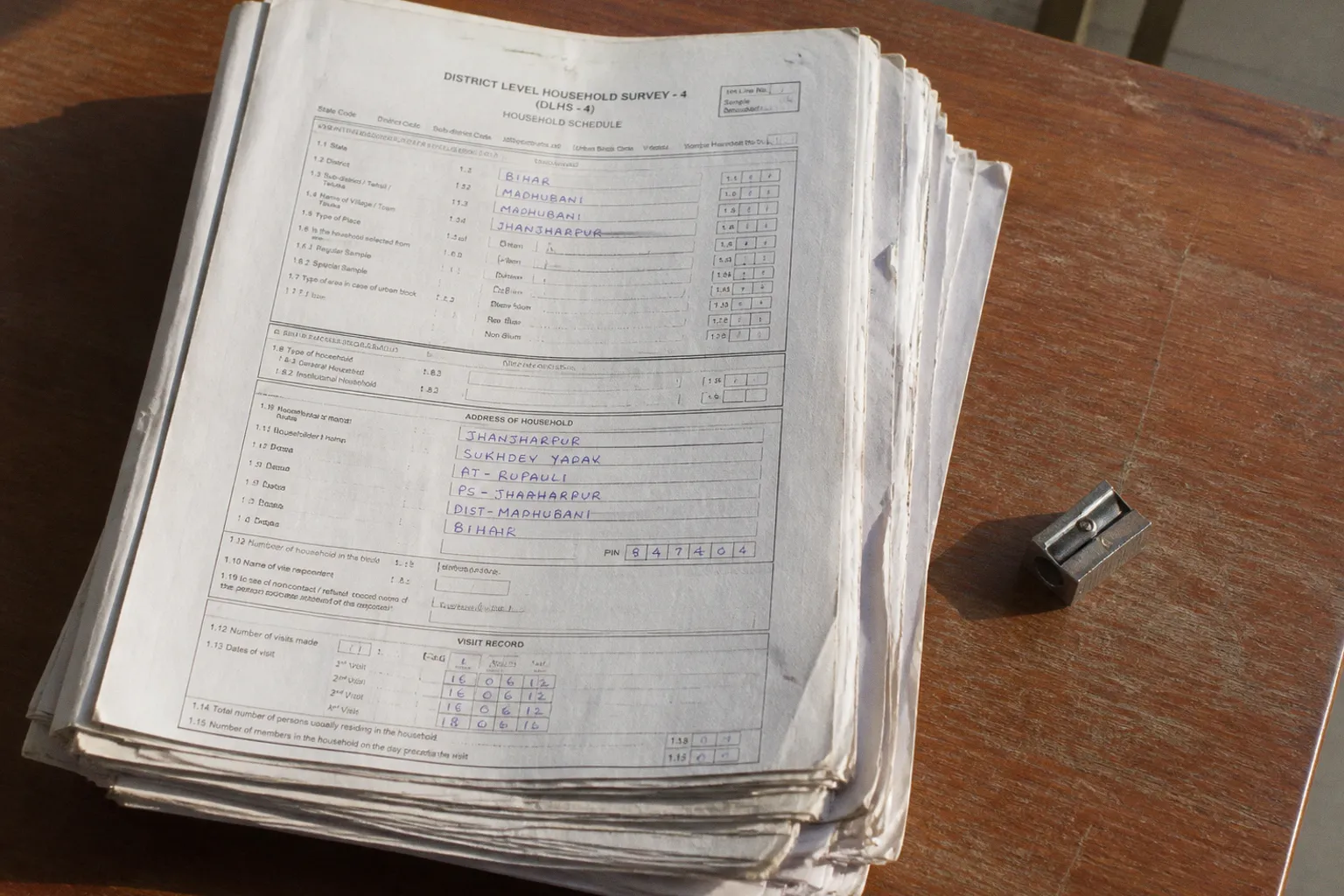
Yet a significant volume of research using DLHS data reports biased estimates or unreliable standard errors—not because the survey was poorly designed, but because analysts treat the weight variables and survey structure as ordinary columns in an ordinary dataset.
The consequences are not abstract. A wrong variance specification can turn a modest association into a seemingly decisive result, or make a meaningful difference appear statistically unimportant. A mistaken interpretation of the weight scale can invalidate totals and complicate comparisons across states. A failure to account for DLHS-4’s geographic coverage can turn a sample-specific estimate into a claim about India as a whole.
This is not a marginal problem confined to student projects. Researchers experienced with Indian survey data still encounter confusion over how the Indian Institute of Population Sciences (IIPS) Mumbai structures its recodes, how state-level normalization works, and which parts of the survey design must be carried into Stata, R, or another statistical package. The documentation exists, but it is distributed across technical appendices, data files, and methodological notes. The result is predictable: analysts spend weeks reverse-engineering the weighting scheme or abandon weights altogether and present unweighted estimates as though they were representative.
The better approach is less dramatic and more exact. Treat the weight as a scaled survey weight, not as a count. Treat the PSU identifier as a component of variance estimation, not as a harmless label. Treat pooled state data as a new analytical problem. And treat representativeness as a property of the sample design, not something that can be restored by pressing the right command.
Decoding the Normalized Weight Variable: The 1,000,000 Factor
The first and most common error in DLHS survey weight application errors concerns the weight variable itself. Standard recode files distributed by IIPS present household and individual weights as integers with no decimal points. That presentation invites an easy but consequential misreading.
A stored value of 3,450 does not mean that the observation represents 3,450 households. Nor does it mean that the value is the actual survey weight divided by 1,000,000. The direction is the other way around: the stored integer is the underlying weight multiplied by 1,000,000. To recover the analysis-scale weight, the stored variable must therefore be divided by 1,000,000.
In notation:
analysis weight = stored weight / 1,000,000
The correction is mechanical:
gen adj_weight = weight / 1000000
The same arithmetic applies in R or Python. The important issue is not the software syntax but the direction of the conversion. A researcher who multiplies the stored value, or interprets it as a population count, is no longer using the weight supplied by the survey design.
It is also important to distinguish a scale error from a relative-weight error. If every observation is multiplied by the same constant, many common estimators retain the same point estimate. A weighted mean is a ratio: the constant appears in both the weighted numerator and the weighted denominator and cancels out. Regression coefficient point estimates in methods that use weights through relative weighting can likewise remain unchanged under uniform rescaling. The absolute scale still matters for totals, and it can matter for variance estimation, degrees-of-freedom conventions, and the interpretation of certain weight types. It is therefore wrong to say that every weighted result is numerically distorted in the same way.
The practical rule remains simple: rescale the stored DLHS variable before analysis and document the operation. That keeps totals interpretable, makes the weight definition visible in the code, and reduces the chance that later analysts will confuse a normalized storage convention with a substantive population quantity.
The most dangerous errors in survey analysis are the ones that produce numbers which look reasonable but reflect the wrong estimand—or the wrong uncertainty.
What the scaling error actually changes
Suppose all weights in a state-level analysis are divided by 1,000,000 before estimation. For a weighted proportion, the numerator and denominator are rescaled together. The proportion itself does not change merely because the common unit has changed. The same is true for many weighted means and for regression coefficient point estimates when the estimator is invariant to a common multiplication of all weights.
That does not make the factor optional. The distinction between point estimates, totals, and variances is central to responsible DLHS data analysis.
- Weighted means and proportions: generally unchanged by a common rescaling of every weight, provided the software and estimator use the weights in a scale-invariant way.
- Regression coefficient point estimates: often unchanged under a uniform rescaling, although the exact behavior depends on the estimation method and how weights are interpreted.
- Population totals: directly affected. A total computed from unrescaled weights can be larger than the intended total by the scaling factor.
- Standard errors and design-based variance: potentially affected, depending on the variance estimator, the type of weight supplied, and the software’s treatment of scale.
- Model fit statistics and likelihood-based quantities: may also depend on the absolute scale, even when coefficient estimates do not.
This is why “the coefficient looked the same” is not a sufficient validation check. A researcher may compare two weighted means, see no difference, and conclude that the scaling was irrelevant. The same file may still generate an unusable population total or a variance estimate based on the wrong weight scale.
The DLHS datasets are designed to be self-weighting at the domain level—urban and rural strata within each state—with household weights further adjusted for individual non-response to produce individual-level weights. The self-weighting property within a domain means that weights may be relatively uniform for a narrowly defined state-by-urban/rural analysis. That uniformity can conceal an error in the scale convention.
A useful validation sequence is therefore broader than comparing one mean before and after rescaling:
1. Inspect the minimum, maximum, mean, and sum of the stored weight.
2. Create the analysis-scale weight by dividing by 1,000,000.
3. Check whether the resulting values are plausible for the intended unit of analysis.
4. Compare weighted and unweighted sample distributions within a known domain.
5. If totals are being estimated, compare them with an external population benchmark appropriate to the same geography and time period.
6. Confirm that household weights are not being used for individual-level outcomes when an individual weight is required.
That last distinction is easy to overlook. A household-level outcome and an individual-level outcome do not necessarily use the same weight. Applying a household weight to an individual fertility, antenatal-care, or child-health measure can introduce a different problem from the 1,000,000 scaling issue. The correct variable depends on the population represented by the observation.
Structuring Complex Survey Designs: Generating Unique Cluster IDs
Survey weights alone do not define the analytical complexity of DLHS data. The survey uses a multi-stage, stratified cluster design. Primary sampling units (PSUs)—typically census villages in rural areas and census enumeration blocks in urban areas—are nested within districts, which are themselves nested within states. The sampling design affects how observations are related to one another, and that relationship is essential for variance estimation.
A survey command that includes weights but ignores clustering is not a full specification of the DLHS design. Nor is a command that includes a PSU variable whose values are only unique within a state or district.
This is the second critical error. In DLHS recode files, cluster identifiers may be numbered within states or districts. Cluster 001 in Rajasthan and cluster 001 in Tamil Nadu are distinct PSUs. If the analyst passes the raw numeric cluster variable to the software without incorporating the relevant geographic identifier, the software may treat those records as belonging to one cluster.
The standard remedy is to construct a globally unique PSU identifier before declaring the survey design:
egen clusterID = group(state cluster)
The precise variables depend on the file and its coding scheme. In some applications, the district must also be included if the cluster code is unique only within districts:
egen clusterID = group(state district cluster)
The principle is more important than the exact command: observations from different PSUs must not be assigned the same cluster ID merely because their local codes match.
Only after checking the identifier should the analyst declare the design. A typical Stata specification might look like:
svyset clusterID [pweight=adj_weight], strata(stratum)
That line is not a universal template. The appropriate weight variable, stratum variable, finite population correction, and single-unit treatment depend on the file and the intended analysis. But it illustrates the order of operations: create the analysis-scale weight, verify the PSU identifier, then specify the design.
What a non-unique PSU identifier affects
A non-unique cluster identifier primarily damages variance estimation. It does not, by itself, alter point estimates when the weights, observations, covariates, and estimation method are otherwise unchanged. The software uses the PSU information to estimate how much observations within clusters resemble one another. If unrelated PSUs are merged, that calculation no longer corresponds to the sample design.
The consequences can include:
- standard errors that are too small or too large;
- confidence intervals with incorrect width;
- design effects that do not describe the actual clustering;
- unreliable test statistics and p-values;
- misleading conclusions about statistical significance.
The direction of the error is not guaranteed. It depends on the pattern of outcomes, the number of clusters, the strata, and the way the erroneous identifier combines observations. A researcher should not assume that duplicate-looking cluster codes always make the analysis more conservative or always inflate significance.
The difference between point estimation and variance estimation should be explicit in the methods section. If the weights and substantive variables remain unchanged, correcting a duplicate PSU code may leave a weighted prevalence or regression coefficient almost exactly where it was. What changes is the estimated uncertainty around that result. This is not a minor technicality: a policy conclusion often depends more on the confidence interval than on the second decimal place of the point estimate.
A basic diagnostic is to examine the mapping between the proposed cluster ID and geography. Each unique PSU should correspond to one sampling unit, while a local cluster code may legitimately appear in several states or districts. Also inspect the number of PSUs and sampled observations within each stratum. Unexpectedly few PSUs, implausibly large clusters, or a cluster spanning unrelated states are signs that the identifier has been built incorrectly.
| Error | Primary statistical consequence | Practical diagnostic |
|---|---|---|
| Failure to divide the stored weight by 1,000,000 | Absolute weight scale is wrong; totals and some variance calculations may be wrong | Compare stored and analysis-scale sums; check a total against a relevant population benchmark |
| Non-unique PSU identifiers | Variance estimation treats unrelated PSUs as one cluster | Cross-tabulate the cluster ID with state and district; verify its geographic uniqueness |
| Ignoring stratification | Design-based variance may be misestimated | Compare results with and without the documented stratum variable |
| Pooling state-normalized weights without adjustment | Pooled estimates do not represent the intended combined population | Examine each state’s contribution to the pooled weighted denominator |
| Using a household weight for an individual outcome | The represented population does not match the estimand | Match the weight to the unit of analysis and outcome definition |
The table is deliberately framed around primary consequences. A single error can have secondary effects, but separating those effects prevents overclaiming. Not every design mistake changes the point estimate, and not every scaling mistake changes a coefficient. Precision in the diagnosis is part of the correction.
Navigating State-Level Normalization and Multi-State Pooling
DLHS weights are normalized at the state level. That is not a design flaw. It is a practical convention that supports analysis within a state and its urban-rural domains. The problem appears when a researcher treats independently normalized state weights as though they were already expressed on one common population scale.
A weight of 500 in Bihar does not necessarily represent the same population quantity as a weight of 500 in Kerala. The stored values can be compared only after the underlying normalization and the target estimand have been understood. If the analyst pools the states and calculates a national or multi-state estimate using the state-normalized weights without adjustment, the contribution of each state may reflect the survey’s normalization scheme rather than the population distribution the estimate is supposed to describe.
This matters most for pooled totals, national percentages, and any analysis in which the relative population size of states is substantively meaningful. It may matter less for an analysis whose estimand is explicitly the average of state-specific estimates, but that is a different estimand and should be labelled as such.
The correction requires an external population standard. The 2011 Census of India provides state-level population totals that can serve as scaling factors for analyses designed to represent that population reference. In broad terms, the analyst calculates a state-specific factor and multiplies the analysis-scale survey weight by it. One way to express the factor is:
state scaling factor = target state population / sum of analysis-scale weights in the state
The exact numerator should match the population represented by the survey file and the target analysis. A household-level file should not automatically be calibrated to a total that refers to individuals, and a women’s or children’s subsample requires a corresponding interpretation. The formula is therefore a framework, not permission to attach any convenient Census number to any file.
The practical work is less elegant than the formula. It requires matching state codes, checking whether the survey geography and the external population geography align, deciding how to handle missing or excluded states, and confirming that the final weighted totals are plausible. Coding discrepancies are especially dangerous because they often do not generate an error message. A state can disappear from the merge, receive a missing factor, or be matched to the wrong population while the analysis continues normally.
Pooling is also a variance problem
Rescaling weights is necessary for a pooled population estimate, but it does not by itself solve the survey-design problem. The pooled analysis still needs valid PSU and stratum identifiers. State identifiers may need to be incorporated into both, depending on how the original codes are defined. A stratum code reused in several states should not be treated as globally unique if the software expects a single identifier across the pooled file.
The analyst should also decide what the pooled result is meant to describe:
- an estimate for the combined population of the included states;
- an average of state-level estimates;
- a model in which state differences are explicitly represented;
- a descriptive estimate for the observed pooled sample only.
These are not interchangeable. The first requires population-scaled weights. The second may require state-specific estimates and an explicit aggregation rule. The third depends on the model and design specification. The fourth should not be described as a national or population-representative estimate without further justification.
Pooling DLHS data across states is not just an append operation. It changes the population reference, the weight interpretation, and the design identifiers at the same time.
Before combining files, document the following:
- the wave and file type;
- the unit represented by each record;
- the weight variable and its scaling convention;
- the population reference used for any rescaling;
- the state and district coding scheme;
- the construction of PSU and stratum identifiers;
- which states and districts are actually present in the pooled sample.
Run the state-specific estimates before the pooled analysis. This gives the researcher a baseline for detecting an implausible pooled result. If one state contributes almost all of the weighted denominator, or if the pooled estimate is identical to the largest state’s result despite substantial data from elsewhere, inspect the rescaling and merge logic before interpreting the substantive finding.
Addressing Representativeness: The DLHS-4 Exclusion Challenge
A structural issue that no amount of correct weighting can resolve affects DLHS-4, the most recent wave in the draft’s comparison, covering 2012–13. DLHS-4 sampled 378,487 households across 321 districts—substantially fewer than DLHS-3’s 720,320 households and 601 districts. Several low-performing states with difficult maternal and child health profiles were excluded from DLHS-4 because they were covered separately by the Annual Health Survey (AHS).
The consequence is categorical: DLHS-4 cannot automatically be treated as a nationally representative survey of the full Indian population. It covers a defined set of districts, not the complete national landscape. A weight can make the sampled districts representative of the population they were designed to represent; it cannot recreate observations from states and districts that are outside the DLHS-4 coverage.
That distinction is often lost when a dataset contains a variable called “weight.” The presence of a weight says something about selection probabilities and adjustment within the covered design. It does not guarantee national coverage. If an analyst labels a DLHS-4 estimate “India” without stating the geographic universe, readers may reasonably assume that the excluded AHS states are included. They are not.
The direction of bias also requires care. It is plausible that excluding states with poorer maternal and child health indicators would make some all-India-looking averages more favorable than the full national picture. But the exact direction and size of bias depend on the outcome, the excluded populations, and the target population. It should not be asserted mechanically for every indicator. For some outcomes, subgroup composition and measurement differences may produce a more complicated pattern.
DLHS-3, covering 2007–08, has the broader national scope used in the draft’s comparison. For analyses requiring national coverage, it is therefore the more appropriate wave among these two, subject to the usual checks on the specific file, outcome, and population. DLHS-4 remains valuable for district-level and covered-area analysis, but its geographic universe must be stated precisely.
Why trend comparisons need a common footprint
The representativeness problem becomes more serious in longitudinal work. A researcher comparing an indicator in DLHS-3 with the corresponding indicator in DLHS-4 is not necessarily comparing the same population at two points in time. The later estimate may reflect both real change and a change in which states and districts are represented.
A defensible comparison can restrict the DLHS-3 data to the geographic footprint shared with DLHS-4, using the same states or districts included in the later wave. That does not remove every comparability problem, but it separates a coverage change from a change in the indicator. The analysis should then report both the geographic restriction and the fact that the comparison is no longer a full DLHS-3 national estimate.
A sound trend analysis should ask:
1. Are the same states and districts included in both waves?
2. Is the outcome defined for the same population and age or parity group?
3. Are the same weight type and survey-design elements being used?
4. Has the earlier wave been restricted to the later wave’s coverage where necessary?
5. Could questionnaire, coding, or fieldwork changes explain part of the observed difference?
6. Are the estimates being compared at the national, state, district, or common-footprint level?
The numbers often look more persuasive when presented as a simple two-wave national trend. The method is more persuasive when the geographic universe is made explicit.
| Parameter | DLHS-3 (2007–08) | DLHS-4 (2012–13) |
|---|---|---|
| Households sampled | 720,320 | 378,487 |
| Districts covered | 601 | 321 |
| National representativeness | Broader national coverage in the comparison | No automatic full-national representativeness; AHS-covered states are excluded from the DLHS-4 frame |
| Weight normalization level | State | State |
| Rescaling for multi-state analysis | Required when the estimand combines state populations | Required when the estimand combines covered state populations |
The table should not be read as saying that DLHS-4 is unusable. It says that the question must match the coverage. “What was the indicator in the DLHS-4 districts?” is answerable with the DLHS-4 data. “What was the indicator in all of India?” requires either an appropriate national source or a carefully justified combination of relevant survey components.
The Risks of Unweighted Analysis in Early DLHS Waves
A recurring pattern in the literature merits direct confrontation. Some researchers, encountering the complexity of DLHS weighting, choose to analyze the data without weights. The justification is usually twofold: the self-weighting property within domains makes unweighted and weighted estimates appear close, and the exact computational methodology used by IIPS to derive weights in early waves—DLHS-1, 1998–99, and DLHS-2, 2002–2004—is less fully documented than the later recodes.
Both points have partial validity. For a narrowly defined domain within a single state, the self-weighting design can make the weighted and unweighted point estimates similar. Documentation for early waves can also be difficult to reconstruct. But neither observation establishes that unweighted analysis is representative.
First, the weights may incorporate non-response adjustments. Even where selection probabilities are relatively uniform within a domain, the achieved sample may not be. Non-response can vary geographically and socioeconomically, and those differences are unlikely to be random with respect to urbanization, literacy, household resources, or access to health services. Those are precisely the factors that matter in reproductive and child health research.
Second, the self-weighting property has boundaries. It should not be extended automatically from a state-specific urban or rural domain to an urban-rural comparison, a district aggregation, a multi-state pool, or a national estimate. Once the analysis crosses domains, the sample allocation and the population composition are no longer interchangeable.
Third, weighting and clustering answer different questions. A researcher may use weights for population representation and the PSU structure for design-based variance. Omitting both because one is uncertain throws away information twice. Conversely, applying weights while reporting ordinary, non-design-based standard errors can make the point estimate look credible while overstating its precision.
Fourth, unweighted results are difficult to compare with weighted results from other studies. An apparent disagreement may reflect different population compositions rather than a genuine substantive contradiction. One paper may describe the observed sample; another may estimate a target population. Without a clear statement of the weighting decision, the reader cannot tell which difference is real.
What to do when the early-wave documentation is incomplete
The defensible response is transparency, not silent omission. Begin by identifying exactly what is known about the file:
- whether the weight is household-level or individual-level;
- whether it is already scaled;
- which population the record represents;
- whether state, district, urban-rural, and non-response adjustments are documented;
- which PSU and stratum variables are available;
- whether the file is intended for descriptive estimates, modelling, or both.
Then conduct sensitivity analysis. Estimate the key outcome with the documented weight and without it, using the same sample and substantive model. If the point estimates are close but the standard errors differ, report that distinction rather than describing the results as simply “robust.” If the estimates diverge across urban and rural domains or states, investigate whether the difference follows the sample allocation or a plausible population composition.
Sensitivity analysis is not a substitute for a weight. It is a way to show how much the conclusion depends on an uncertain design element. The paper should state which specification is treated as primary, why, and what limitation remains. If the weight cannot be verified at all, use cautious language: describe the analysis as sample-based or exploratory rather than presenting it as a representative population estimate.
The same discipline applies to regression. A weighted regression coefficient can remain close to an unweighted coefficient even when the weighted prevalence differs, particularly when the covariate relationships are stable across sampled groups. That does not prove that the unweighted model is representative. It only says that the coefficient for that model is not highly sensitive to the weighting choice. The target population, standard errors, and marginal predictions may still differ.
A Workflow That Prevents Rework
Most wasted research time comes from discovering design problems after the tables and models have already been built. A short sequence at the beginning is more efficient than repairing a manuscript at the end.
Start with the observation, not the command
Identify whether each row represents a household, a woman, a child, a birth, or another unit. Match the outcome to the relevant weight. Confirm that duplicate records are expected—for example, several children within a household or several births reported by one woman—and do not mistake the resulting structure for a data-entry error.
Decode and preserve the original weight
Keep the original stored variable unchanged. Create a separate analysis-scale variable by dividing it by 1,000,000 when that is the documented convention. Record the transformation in the do-file or analysis script. Do not overwrite the source variable with an unexplained decimal version.
Inspect geography and design variables
Check state, district, urban-rural domain, stratum, and cluster fields before using them in a survey declaration. Look for codes reused across geographic units. Build composite identifiers where needed, and verify them with cross-tabulations. A unique identifier should be tested, not assumed.
Separate state-specific from pooled analysis
Produce state-specific descriptive results first. If the analysis is pooled, define the target population and rescale the weights to a common population standard. Do not describe an equal contribution from each state as a national estimate unless that equal-state estimand is actually the research question.
Validate both estimates and uncertainty
Compare weighted and unweighted point estimates, but also inspect standard errors, confidence intervals, design effects, and effective sample sizes. A plausible prevalence with an implausibly narrow interval is a design warning, not evidence of precision.
Write the geographic universe into the result
For DLHS-4, state exactly which states or districts are represented. For trend work, say whether the earlier wave was restricted to the later wave’s footprint. For pooled work, name the population standard used for rescaling. These details belong in the analysis description, not in a footnote added after peer review.
Closing the Methodological Gap
The District Level Household Survey remains one of the most granular demographic datasets available for India’s reproductive and child health landscape. Four waves spanning 1998 to 2013 provide longitudinal depth, while the district-level design offers a resolution that many international demographic health surveys cannot match. Its usefulness is precisely why careless analysis is costly. Findings from DLHS data are often used to compare states, identify underserved districts, and evaluate health-system priorities. The analytical frame travels with the number.
The core corrections are straightforward, but they must be applied to the right problem. Divide the stored weight by 1,000,000 to recover the analysis-scale value. Do not claim that a uniform rescaling necessarily changes every weighted mean or regression coefficient; distinguish point estimates from totals and variance calculations. Construct globally meaningful PSU identifiers so that variance estimation follows the sample design. Do not imply that correcting a cluster ID will materially change a point estimate when the weights and observations are unchanged. Rescale state-normalized weights before making a pooled population claim. And do not use a technically correct weight to manufacture national representativeness for DLHS-4.
The unweighted shortcut deserves the same measured treatment. It is not automatically disastrous in every narrow, within-domain comparison, but it is not a defensible default for representative estimates. When early-wave documentation is incomplete, sensitivity analysis and explicit limitations are stronger than false certainty.
The research community does not need an exotic statistical method for DLHS data. It needs a clean distinction between the population being estimated, the unit represented by each record, the scale of the weight, and the part of the design that governs uncertainty. Once those distinctions are made, the software commands are rarely the difficult part.
A well-specified DLHS analysis can stand up to replication and policy scrutiny. An analysis that treats a scaled weight as a count, a local cluster code as a global PSU, or a covered subset as the whole country wastes more than research time. It obscures the population the data were collected to describe.